Due to the fact that random measurement errors always occur, one can
observe replicate measurements to differ slightly. This deviation from a central
value (usually taken to be the 'true' value) can be summarized by a histogram. A
histogram shows the (relative) frequency of each measurement.
Practical results
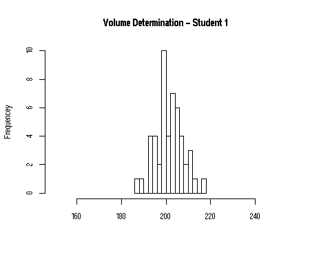
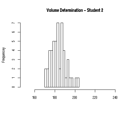
In the figure below you see the
practical results of two chemistry students pipetting a volume of 50 x 200 µL
with a
P1000 pipet (a pipet with a volume of 1000 µL). As you can see, there is considerable spread in the results. However,
values close to the true value of 200 µL are more often found than
values far
away for student 1. On the other hand, student 2 finds consistently lower values than the
other student.
Question: which results are more precise and which are more
accurate?
Histograms can be very useful to summarize the spread in the data. In
many cases, the spread in the data can also be described by a normal
distribution. Put differently: random experimental errors show a normal
distribution. If the number of experiments is large enough, the histogram
approximates the (smoother) shape of a normal distribution.
The normal distribution is characterised by two parameters:
the mean and the standard deviation. With these, we
can calculate the theoretical normal distribution (or
Gauss-curve). When you fill in values for mean and
standard deviation, two new plots will appear. In the right plot,
the scale of the figure will remain as it is, showing the change
of the curve relative to the original situation. The left plot
contains the same data but will show you the 'optimally scaled' plot.
- What is the effect on the Gauss-curve of changing the
mean? Try a few values.
- What is the effect of changing the standard deviation?
Try a few values.
Theory and experiment
If we calculate values for the mean and the standard deviation of another data set,
containing titration data, we obtain the corresponding Gauss curve shown below:
The agreement is not very good, because the number of titrations is
quite small. When we perform more experiments, the results will be
more like the theoretical distribution. You can see that by simulating
a number of experiments and comparing theory and experiment: